Introduction to EDA - Coverage Type
About
This is the part of the R code for the CAP394 - Introduction to Data Science course.
In this document we'll do some Exploratory Data Analysis on the Covertype Data Set.
From the data source:
Predicting forest cover type from cartographic variables only (no remotely sensed data). The actual forest cover type for a given observation (30 x 30 meter cell) was determined from US Forest Service (USFS) Region 2 Resource Information System (RIS) data. Independent variables were derived from data originally obtained from US Geological Survey (USGS) and USFS data. Data is in raw form (not scaled) and contains binary (0 or 1) columns of data for qualitative independent variables (wilderness areas and soil types).
This study area includes four wilderness areas located in the Roosevelt National Forest of northern Colorado. These areas represent forests with minimal human-caused disturbances, so that existing forest cover types are more a result of ecological processes rather than forest management practices.
Some background information for these four wilderness areas: Neota (area 2) probably has the highest mean elevational value of the 4 wilderness areas. Rawah (area 1) and Comanche Peak (area 3) would have a lower mean elevational value, while Cache la Poudre (area 4) would have the lowest mean elevational value.
As for primary major tree species in these areas, Neota would have spruce/fir (type 1), while Rawah and Comanche Peak would probably have lodgepole pine (type 2) as their primary species, followed by spruce/fir and aspen (type 5). Cache la Poudre would tend to have Ponderosa pine (type 3), Douglas-fir (type 6), and cottonwood/willow (type 4).
The Rawah and Comanche Peak areas would tend to be more typical of the overall dataset than either the Neota or Cache la Poudre, due to their assortment of tree species and range of predictive variable values (elevation, etc.) Cache la Poudre would probably be more unique than the others, due to its relatively low elevation range and species composition.
Initial Settings
Let's assume that the data file is stored locally, then let's load it as a data frame. The data file is a CSV file, but without header, so we need to provide the attributes' names.
covtype <- read.csv(file="Data/CoverageType/covtype.data", header=FALSE, sep=",", stringsAsFactors=FALSE)
head(covtype,n = 2)
##     V1 V2 V3  V4 V5  V6  V7  V8  V9  V10 V11 V12 V13 V14 V15 V16 V17 V18
## 1 2596 51  3 258  0 510 221 232 148 6279   1   0   0   0   0   0   0   0
## 2 2590 56  2 212 -6 390 220 235 151 6225   1   0   0   0   0   0   0   0
##   V19 V20 V21 V22 V23 V24 V25 V26 V27 V28 V29 V30 V31 V32 V33 V34 V35 V36
## 1   0   0   0   0   0   0   0   0   0   0   0   0   0   0   0   0   0   0
## 2   0   0   0   0   0   0   0   0   0   0   0   0   0   0   0   0   0   0
##   V37 V38 V39 V40 V41 V42 V43 V44 V45 V46 V47 V48 V49 V50 V51 V52 V53 V54
## 1   0   0   0   0   0   0   1   0   0   0   0   0   0   0   0   0   0   0
## 2   0   0   0   0   0   0   1   0   0   0   0   0   0   0   0   0   0   0
##   V55
## 1   5
## 2   5
All variables have generic names, let's name them correctly. The information was taken from the file , which can also be downloaded from the UCI Machine Learning Repository
# "Fixed" attributes' names
names <- c("Elevation","Aspect","Slope","HorDistToHydro","VertDistToHydro",
           "HorDistRoad","Hillshade09","Hillshade12","Hillshade15",
           "HorDistFire")
# Four binary attributes for wilderness areas:
names <- c(names,"WA_RWA","WA_NWA","WA_CPWA","WA_CLPWA")
# 40 (!) binary attributes for soil types:
names <- c(names,sprintf("ST%02d",1:40))
# The cover type
names <- c(names,"Class")
# Assign these names to the attributes
names(covtype) <- names
# Let's also assign labels to the coverage types.
covtype$Class <- as.factor(covtype$Class)
levels(covtype$Class) <- c("Spruce/Fir", "Lodgepole Pine",
                           "Ponderosa Pine","Cottonwood/Willow","Aspen",
                           "Douglas-fir","Krummholz")
# How does it looks like?
str(covtype)
## 'data.frame':	581012 obs. of  55 variables:
##  $ Elevation      : int  2596 2590 2804 2785 2595 2579 2606 2605 2617 2612 ...
##  $ Aspect         : int  51 56 139 155 45 132 45 49 45 59 ...
##  $ Slope          : int  3 2 9 18 2 6 7 4 9 10 ...
##  $ HorDistToHydro : int  258 212 268 242 153 300 270 234 240 247 ...
##  $ VertDistToHydro: int  0 -6 65 118 -1 -15 5 7 56 11 ...
##  $ HorDistRoad    : int  510 390 3180 3090 391 67 633 573 666 636 ...
##  $ Hillshade09    : int  221 220 234 238 220 230 222 222 223 228 ...
##  $ Hillshade12    : int  232 235 238 238 234 237 225 230 221 219 ...
##  $ Hillshade15    : int  148 151 135 122 150 140 138 144 133 124 ...
##  $ HorDistFire    : int  6279 6225 6121 6211 6172 6031 6256 6228 6244 6230 ...
##  $ WA_RWA         : int  1 1 1 1 1 1 1 1 1 1 ...
##  $ WA_NWA         : int  0 0 0 0 0 0 0 0 0 0 ...
##  $ WA_CPWA        : int  0 0 0 0 0 0 0 0 0 0 ...
##  $ WA_CLPWA       : int  0 0 0 0 0 0 0 0 0 0 ...
##  $ ST01           : int  0 0 0 0 0 0 0 0 0 0 ...
##  $ ST02           : int  0 0 0 0 0 0 0 0 0 0 ...
##  $ ST03           : int  0 0 0 0 0 0 0 0 0 0 ...
##  $ ST04           : int  0 0 0 0 0 0 0 0 0 0 ...
##  $ ST05           : int  0 0 0 0 0 0 0 0 0 0 ...
##  $ ST06           : int  0 0 0 0 0 0 0 0 0 0 ...
##  $ ST07           : int  0 0 0 0 0 0 0 0 0 0 ...
##  $ ST08           : int  0 0 0 0 0 0 0 0 0 0 ...
##  $ ST09           : int  0 0 0 0 0 0 0 0 0 0 ...
##  $ ST10           : int  0 0 0 0 0 0 0 0 0 0 ...
##  $ ST11           : int  0 0 0 0 0 0 0 0 0 0 ...
##  $ ST12           : int  0 0 1 0 0 0 0 0 0 0 ...
##  $ ST13           : int  0 0 0 0 0 0 0 0 0 0 ...
##  $ ST14           : int  0 0 0 0 0 0 0 0 0 0 ...
##  $ ST15           : int  0 0 0 0 0 0 0 0 0 0 ...
##  $ ST16           : int  0 0 0 0 0 0 0 0 0 0 ...
##  $ ST17           : int  0 0 0 0 0 0 0 0 0 0 ...
##  $ ST18           : int  0 0 0 0 0 0 0 0 0 0 ...
##  $ ST19           : int  0 0 0 0 0 0 0 0 0 0 ...
##  $ ST20           : int  0 0 0 0 0 0 0 0 0 0 ...
##  $ ST21           : int  0 0 0 0 0 0 0 0 0 0 ...
##  $ ST22           : int  0 0 0 0 0 0 0 0 0 0 ...
##  $ ST23           : int  0 0 0 0 0 0 0 0 0 0 ...
##  $ ST24           : int  0 0 0 0 0 0 0 0 0 0 ...
##  $ ST25           : int  0 0 0 0 0 0 0 0 0 0 ...
##  $ ST26           : int  0 0 0 0 0 0 0 0 0 0 ...
##  $ ST27           : int  0 0 0 0 0 0 0 0 0 0 ...
##  $ ST28           : int  0 0 0 0 0 0 0 0 0 0 ...
##  $ ST29           : int  1 1 0 0 1 1 1 1 1 1 ...
##  $ ST30           : int  0 0 0 1 0 0 0 0 0 0 ...
##  $ ST31           : int  0 0 0 0 0 0 0 0 0 0 ...
##  $ ST32           : int  0 0 0 0 0 0 0 0 0 0 ...
##  $ ST33           : int  0 0 0 0 0 0 0 0 0 0 ...
##  $ ST34           : int  0 0 0 0 0 0 0 0 0 0 ...
##  $ ST35           : int  0 0 0 0 0 0 0 0 0 0 ...
##  $ ST36           : int  0 0 0 0 0 0 0 0 0 0 ...
##  $ ST37           : int  0 0 0 0 0 0 0 0 0 0 ...
##  $ ST38           : int  0 0 0 0 0 0 0 0 0 0 ...
##  $ ST39           : int  0 0 0 0 0 0 0 0 0 0 ...
##  $ ST40           : int  0 0 0 0 0 0 0 0 0 0 ...
##  $ Class          : Factor w/ 7 levels "Spruce/Fir","Lodgepole Pine",..: 5 5 2 2 5 2 5 5 5 5 ...
Can we make sure that there isn't more than one wilderness area in each record? Here's one of several possible ways to do that.
countWA <- covtype$WA_RWA + covtype$WA_NWA + covtype$WA_CPWA + covtype$WA_CLPWA
paste(min(countWA),max(countWA))
## [1] "1 1"
Good -- there is one and only one of (covtype$WA_RWA, covtype$WA_NWA, covtype$WA_CPWA, covtype$WA_CLPWA) for each row. What about the soil types?
soilT <- sprintf("ST%02d",1:40)
countST <- rowSums(covtype[,soilT])
paste(min(countST),max(countST))
## [1] "1 1"
There is also one and only one of (covtype$ST01 .. covtype$ST40) for each row. So now we made sure that these binary variables are indicators of the wilderness area and soil types, only one variable for each of those is set to one, and the others to zero. Let's reorganize the dataset to make it more concise.
Converting binary variables to a single categorical one (factor)
Let's convert the binary representation used to represent one of the wilderness areas to a single code for that wilderness area. We need to locate the position of the value 1 in each of the four attributes that corresponds to the wilderness area, then convert it to a factor:
# Which are the columns we want to consider?
searchOn <- c("WA_RWA","WA_NWA","WA_CPWA","WA_CLPWA")
# Get the index of each WA_
indexOfWA <- apply(covtype[,searchOn], 1, function(x) which(x == 1))
# Convert it to a factor with the column names we used.
factorOfWA <- factor(indexOfWA,labels = searchOn)
# Add it to the data frame
covtype$WildArea <- factorOfWA
# Drop the binary variables we don't need anymore
covtype[searchOn] <- list(NULL)
Now let's do the same for the coverage types:
# Which are the columns we want to consider?
searchOn <- sprintf("ST%02d",1:40)
searchOn
##  [1] "ST01" "ST02" "ST03" "ST04" "ST05" "ST06" "ST07" "ST08" "ST09" "ST10"
## [11] "ST11" "ST12" "ST13" "ST14" "ST15" "ST16" "ST17" "ST18" "ST19" "ST20"
## [21] "ST21" "ST22" "ST23" "ST24" "ST25" "ST26" "ST27" "ST28" "ST29" "ST30"
## [31] "ST31" "ST32" "ST33" "ST34" "ST35" "ST36" "ST37" "ST38" "ST39" "ST40"
# Get the index of 1 in ST01..ST40
indexOfST <- apply(covtype[,searchOn], 1, function(x) which(x == 1))
# Convert it to a factor with the column names we used.
factorOfST <- factor(indexOfST,labels = searchOn)
# Add it to the data frame
covtype$SoilType <- factorOfST
# Drop the binary variables we don't need anymore
covtype[searchOn] <- list(NULL)
str(covtype)
## 'data.frame':	581012 obs. of  13 variables:
##  $ Elevation      : int  2596 2590 2804 2785 2595 2579 2606 2605 2617 2612 ...
##  $ Aspect         : int  51 56 139 155 45 132 45 49 45 59 ...
##  $ Slope          : int  3 2 9 18 2 6 7 4 9 10 ...
##  $ HorDistToHydro : int  258 212 268 242 153 300 270 234 240 247 ...
##  $ VertDistToHydro: int  0 -6 65 118 -1 -15 5 7 56 11 ...
##  $ HorDistRoad    : int  510 390 3180 3090 391 67 633 573 666 636 ...
##  $ Hillshade09    : int  221 220 234 238 220 230 222 222 223 228 ...
##  $ Hillshade12    : int  232 235 238 238 234 237 225 230 221 219 ...
##  $ Hillshade15    : int  148 151 135 122 150 140 138 144 133 124 ...
##  $ HorDistFire    : int  6279 6225 6121 6211 6172 6031 6256 6228 6244 6230 ...
##  $ Class          : Factor w/ 7 levels "Spruce/Fir","Lodgepole Pine",..: 5 5 2 2 5 2 5 5 5 5 ...
##  $ WildArea       : Factor w/ 4 levels "WA_RWA","WA_NWA",..: 1 1 1 1 1 1 1 1 1 1 ...
##  $ SoilType       : Factor w/ 40 levels "ST01","ST02",..: 29 29 12 30 29 29 29 29 29 29 ...
A warning: the code to convert binary matrices to a factor work only if there is at least one and only one "1" value for a category. When testing this code I used a subset of the dataset and ran into errors like Error in factor(indexOfST, labels = searchOn): invalid 'labels'; length 40 should be 1 or 27, since not all indexes between 1 and 40 were found in the subset of the original dataset?.
EDA with this dataset
First, a summary of the attributes:
summary(covtype)
##    Elevation        Aspect          Slope      HorDistToHydro
##  Min.   :1859   Min.   :  0.0   Min.   : 0.0   Min.   :   0.0
##  1st Qu.:2809   1st Qu.: 58.0   1st Qu.: 9.0   1st Qu.: 108.0
##  Median :2996   Median :127.0   Median :13.0   Median : 218.0
##  Mean   :2959   Mean   :155.7   Mean   :14.1   Mean   : 269.4
##  3rd Qu.:3163   3rd Qu.:260.0   3rd Qu.:18.0   3rd Qu.: 384.0
##  Max.   :3858   Max.   :360.0   Max.   :66.0   Max.   :1397.0
##
##  VertDistToHydro    HorDistRoad    Hillshade09     Hillshade12
##  Min.   :-173.00   Min.   :   0   Min.   :  0.0   Min.   :  0.0
##  1st Qu.:   7.00   1st Qu.:1106   1st Qu.:198.0   1st Qu.:213.0
##  Median :  30.00   Median :1997   Median :218.0   Median :226.0
##  Mean   :  46.42   Mean   :2350   Mean   :212.1   Mean   :223.3
##  3rd Qu.:  69.00   3rd Qu.:3328   3rd Qu.:231.0   3rd Qu.:237.0
##  Max.   : 601.00   Max.   :7117   Max.   :254.0   Max.   :254.0
##
##   Hillshade15     HorDistFire                 Class
##  Min.   :  0.0   Min.   :   0   Spruce/Fir       :211840
##  1st Qu.:119.0   1st Qu.:1024   Lodgepole Pine   :283301
##  Median :143.0   Median :1710   Ponderosa Pine   : 35754
##  Mean   :142.5   Mean   :1980   Cottonwood/Willow:  2747
##  3rd Qu.:168.0   3rd Qu.:2550   Aspen            :  9493
##  Max.   :254.0   Max.   :7173   Douglas-fir      : 17367
##                                 Krummholz        : 20510
##      WildArea         SoilType
##  WA_RWA  :260796   ST29   :115247
##  WA_NWA  : 29884   ST23   : 57752
##  WA_CPWA :253364   ST32   : 52519
##  WA_CLPWA: 36968   ST33   : 45154
##                    ST22   : 33373
##                    ST10   : 32634
##                    (Other):244333
# Let's save it just in case!
save(covtype,file="Data/CoverageType/CovType2.R")
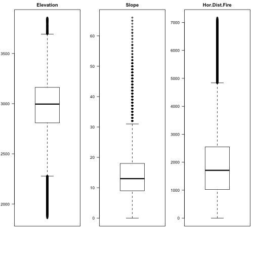
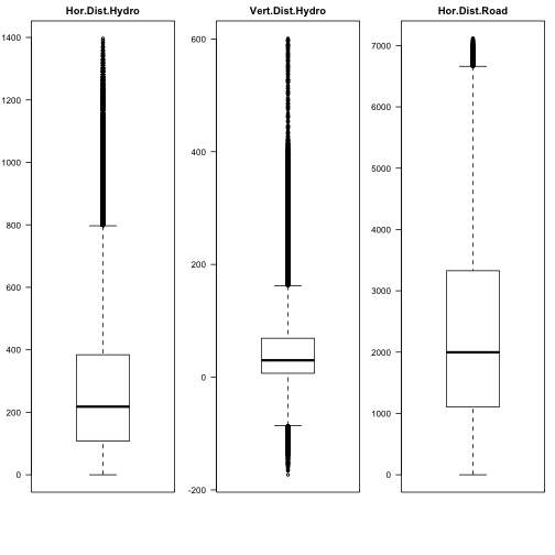
Let's see boxplots of some attributes:
par(mfrow=c(1,3),mar=c(6,3,2,1))
boxplot(covtype$Elevation, main="Elevation",las=2)
boxplot(covtype$Slope, main="Slope",las=2)
boxplot(covtype$HorDistFire, main="Hor.Dist.Fire",las=2)
par(mfrow=c(1,3),mar=c(6,3,2,1))
boxplot(covtype$HorDistToHydro, main="Hor.Dist.Hydro",las=2)
boxplot(covtype$VertDistToHydro, main="Vert.Dist.Hydro",las=2)
boxplot(covtype$HorDistRoad, main="Hor.Dist.Road",las=2)
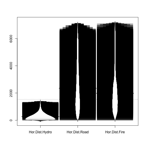
Let's see a beanplot plot of some of those attributes.
library(beanplot)
beanplot(covtype$HorDistToHydro,covtype$HorDistRoad,covtype$HorDistFire,
        names=c("Hor.Dist.Hydro","Hor.Dist.Road","Hor.Dist.Fire"))
Several measures are factors: how do they compare to each other?
library(xtable)
tabSW <- table(covtype$SoilType,covtype$WildArea)
print(xtable(tabSW), type="html")
| WA_RWA | WA_NWA | WA_CPWA | WA_CLPWA | |
|---|---|---|---|---|
| ST01 | 0 | 0 | 0 | 3031 |
| ST02 | 0 | 0 | 5381 | 2144 |
| ST03 | 0 | 0 | 2368 | 2455 |
| ST04 | 0 | 0 | 11158 | 1238 |
| ST05 | 0 | 0 | 0 | 1597 |
| ST06 | 0 | 0 | 0 | 6575 |
| ST07 | 105 | 0 | 0 | 0 |
| ST08 | 179 | 0 | 0 | 0 |
| ST09 | 1147 | 0 | 0 | 0 |
| ST10 | 0 | 0 | 14720 | 17914 |
| ST11 | 0 | 0 | 11814 | 596 |
| ST12 | 29971 | 0 | 0 | 0 |
| ST13 | 0 | 255 | 17176 | 0 |
| ST14 | 0 | 0 | 240 | 359 |
| ST15 | 0 | 0 | 0 | 3 |
| ST16 | 2140 | 117 | 325 | 263 |
| ST17 | 0 | 0 | 2629 | 793 |
| ST18 | 1829 | 70 | 0 | 0 |
| ST19 | 2749 | 597 | 675 | 0 |
| ST20 | 6752 | 55 | 2452 | 0 |
| ST21 | 0 | 0 | 838 | 0 |
| ST22 | 19648 | 5363 | 8362 | 0 |
| ST23 | 28528 | 8153 | 21071 | 0 |
| ST24 | 2903 | 2123 | 16252 | 0 |
| ST25 | 0 | 474 | 0 | 0 |
| ST26 | 0 | 0 | 2589 | 0 |
| ST27 | 0 | 0 | 1086 | 0 |
| ST28 | 0 | 0 | 946 | 0 |
| ST29 | 115173 | 74 | 0 | 0 |
| ST30 | 30170 | 0 | 0 | 0 |
| ST31 | 0 | 426 | 25240 | 0 |
| ST32 | 0 | 3761 | 48758 | 0 |
| ST33 | 0 | 2817 | 42337 | 0 |
| ST34 | 0 | 0 | 1611 | 0 |
| ST35 | 656 | 503 | 732 | 0 |
| ST36 | 0 | 0 | 119 | 0 |
| ST37 | 232 | 0 | 66 | 0 |
| ST38 | 7507 | 2073 | 5993 | 0 |
| ST39 | 6758 | 931 | 6117 | 0 |
| ST40 | 4349 | 2092 | 2309 | 0 |
tabCW <- table(covtype$Class,covtype$WildArea)
print(xtable(tabCW), type="html")
| WA_RWA | WA_NWA | WA_CPWA | WA_CLPWA | |
|---|---|---|---|---|
| Spruce/Fir | 105717 | 18595 | 87528 | 0 |
| Lodgepole Pine | 146197 | 8985 | 125093 | 3026 |
| Ponderosa Pine | 0 | 0 | 14300 | 21454 |
| Cottonwood/Willow | 0 | 0 | 0 | 2747 |
| Aspen | 3781 | 0 | 5712 | 0 |
| Douglas-fir | 0 | 0 | 7626 | 9741 |
| Krummholz | 5101 | 2304 | 13105 | 0 |
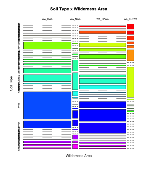
It is possible to visualize the tables, but this may not be very helpful in this case.
colfunc <- colorRampPalette(c("red", "yellow","green","cyan","blue","magenta"))
mosaicplot(t(tabSW),main="Soil Type x Wilderness Area",
              ylab="Soil Type",xlab="Wilderness Area",col=colfunc(nlevels(covtype$SoilType)))
mosaicplot(t(tabCW),main="Class x Wilderness Area",
              ylab="Class",xlab="Wilderness Area",col=colfunc(nlevels(covtype$Class)))
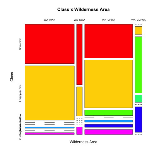
Note that we "rotated" (transposed) the tables for better results.
From the covtype.info file: As for primary major tree species in these areas, Neota would have spruce/fir (type 1), while Rawah and Comanche Peak would probably have lodgepole pine (type 2) as their primary species, followed by spruce/fir and aspen (type 5). Cache la Poudre would tend to have Ponderosa pine (type 3), Douglas-fir (type 6), and cottonwood/willow (type 4).
Enriching the data
The covtype.info contains information on how to map the soil type to one of the USFS Ecological Landtype Units (ELUs), and from there to climatic and geologic zones. Some manual coding would be required to convert the information on covtype.info to tables for climatic and geological zones and to create contingency tables between those tables.
References
- https://archive.ics.uci.edu/ml/datasets/Covertype
- https://stackoverflow.com/questions/28233561/finding-rows-containing-a-value-or-values-in-any-column
- https://stackoverflow.com/questions/32052723/sum-all-columns-whose-names-start-with-a-pattern-by-group
- https://stackoverflow.com/questions/18587334/subset-data-to-contain-only-columns-whose-names-match-a-condition
- https://stackoverflow.com/questions/5234117/how-to-drop-columns-by-name-in-a-data-frame
- http://www.cyclismo.org/tutorial/R/intermediatePlotting.html#mosaic-plot
- https://stackoverflow.com/questions/15282580/how-to-generate-a-number-of-most-distinctive-colors-in-r
Warning: Code and results presented on this document are for reference use only. Code was written to be clear, not efficient. There are several ways to achieve the results, not all were considered.
See the R source code for this notebook.