Data Science Example - Iris dataset
About
This is an example of a notebook to demonstrate concepts of Data Science. In this example we will do some exploratory data analysis on the famous Iris dataset.
The Iris Dataset contains four features (length and width of sepals and petals) of 50 samples of three species of Iris (Iris setosa, Iris virginica and Iris versicolor). These measures were used to create a linear discriminant model to classify the species. The dataset is often used in data mining, classification and clustering examples and to test algorithms.
Information about the original paper and usages of the dataset can be found in the UCI Machine Learning Repository -- Iris Data Set.
Just for reference, here are pictures of the three flowers species:
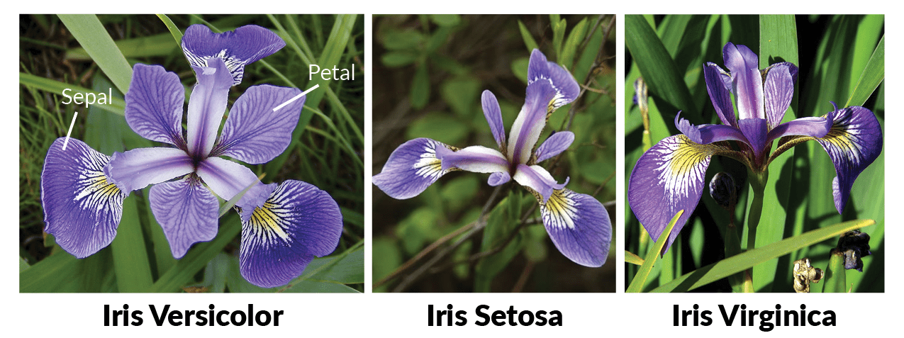
from Machine Learning in R for beginners
The Data
It is possible to download the data from the UCI Machine Learning Repository -- Iris Data Set, but the datasets library in R already contains it. Just by loading the library, a data frame named iris will be made available and can be used straight away:
library(datasets)
str(iris)
## 'data.frame':	150 obs. of  5 variables:
##  $ Sepal.Length: num  5.1 4.9 4.7 4.6 5 5.4 4.6 5 4.4 4.9 ...
##  $ Sepal.Width : num  3.5 3 3.2 3.1 3.6 3.9 3.4 3.4 2.9 3.1 ...
##  $ Petal.Length: num  1.4 1.4 1.3 1.5 1.4 1.7 1.4 1.5 1.4 1.5 ...
##  $ Petal.Width : num  0.2 0.2 0.2 0.2 0.2 0.4 0.3 0.2 0.2 0.1 ...
##  $ Species     : Factor w/ 3 levels "setosa","versicolor",..: 1 1 1 1 1 1 1 1 1 1 ...
Let's take a look at the data itself. Let's see the first 5 rows of data for each class:
# Get first 5 rows of each subset
subset(iris, Species == "setosa")[1:5,]
##   Sepal.Length Sepal.Width Petal.Length Petal.Width Species
## 1          5.1         3.5          1.4         0.2  setosa
## 2          4.9         3.0          1.4         0.2  setosa
## 3          4.7         3.2          1.3         0.2  setosa
## 4          4.6         3.1          1.5         0.2  setosa
## 5          5.0         3.6          1.4         0.2  setosa
subset(iris, Species == "versicolor")[1:5,]
##    Sepal.Length Sepal.Width Petal.Length Petal.Width    Species
## 51          7.0         3.2          4.7         1.4 versicolor
## 52          6.4         3.2          4.5         1.5 versicolor
## 53          6.9         3.1          4.9         1.5 versicolor
## 54          5.5         2.3          4.0         1.3 versicolor
## 55          6.5         2.8          4.6         1.5 versicolor
subset(iris, Species == "virginica")[1:5,]
##     Sepal.Length Sepal.Width Petal.Length Petal.Width   Species
## 101          6.3         3.3          6.0         2.5 virginica
## 102          5.8         2.7          5.1         1.9 virginica
## 103          7.1         3.0          5.9         2.1 virginica
## 104          6.3         2.9          5.6         1.8 virginica
## 105          6.5         3.0          5.8         2.2 virginica
Exploratory Data Analysis
A quick look at the data shows that Petal.Length of class setosa is shorter than the Petal.Length of other classes -- is that true?
# Get column "Species" for all lines where Petal.Length < 2
subset(iris, Petal.Length < 2)[,"Species"]
##  [1] setosa setosa setosa setosa setosa setosa setosa setosa setosa setosa
## [11] setosa setosa setosa setosa setosa setosa setosa setosa setosa setosa
## [21] setosa setosa setosa setosa setosa setosa setosa setosa setosa setosa
## [31] setosa setosa setosa setosa setosa setosa setosa setosa setosa setosa
## [41] setosa setosa setosa setosa setosa setosa setosa setosa setosa setosa
## Levels: setosa versicolor virginica
Cool, we have a first model that helps explain part of our data!
We want to learn more about the data. We can calculate basic statistics on each of the data frame's columns with summary:
summary(iris)
##   Sepal.Length    Sepal.Width     Petal.Length    Petal.Width
##  Min.   :4.300   Min.   :2.000   Min.   :1.000   Min.   :0.100
##  1st Qu.:5.100   1st Qu.:2.800   1st Qu.:1.600   1st Qu.:0.300
##  Median :5.800   Median :3.000   Median :4.350   Median :1.300
##  Mean   :5.843   Mean   :3.057   Mean   :3.758   Mean   :1.199
##  3rd Qu.:6.400   3rd Qu.:3.300   3rd Qu.:5.100   3rd Qu.:1.800
##  Max.   :7.900   Max.   :4.400   Max.   :6.900   Max.   :2.500
##        Species
##  setosa    :50
##  versicolor:50
##  virginica :50
##
##
##
Numbers can tell a lot, but sometimes it is better to see the statistics with boxplots.
par(mar=c(7,5,1,1)) # more space to labels
boxplot(iris,las=2)

Here's how to interpret a boxplot:

This gives us a rough estimate of the distribution of the values for each attribute. But maybe it makes more sense to see the distribution of the values considering each class, since we have labels for each class.
irisVer <- subset(iris, Species == "versicolor")
irisSet <- subset(iris, Species == "setosa")
irisVir <- subset(iris, Species == "virginica")
par(mfrow=c(1,3),mar=c(6,3,2,1))
boxplot(irisVer[,1:4], main="Versicolor",ylim = c(0,8),las=2)
boxplot(irisSet[,1:4], main="Setosa",ylim = c(0,8),las=2)
boxplot(irisVir[,1:4], main="Virginica",ylim = c(0,8),las=2)

Histograms (which should be calculated per attribute) are also very useful:
hist(iris$Petal.Length)

Let's see the histograms of one particular attribute, one for each class:
par(mfrow=c(1,3))
hist(irisVer$Petal.Length,breaks=seq(0,8,l=17),xlim=c(0,8),ylim=c(0,40))
hist(irisSet$Petal.Length,breaks=seq(0,8,l=17),xlim=c(0,8),ylim=c(0,40))
hist(irisVir$Petal.Length,breaks=seq(0,8,l=17),xlim=c(0,8),ylim=c(0,40))

These show that the distribution of values for Petal.Length are different for each class.
Bean plots shows the data and its distribution:
library(beanplot)
xiris <- iris
xiris$Species <- NULL
beanplot(xiris, main = "Iris flowers",col=c('#ff8080','#0000FF','#0000FF','#FF00FF'), border = "#000000")

Note: I used violin plots for some versions of this document, but I cannot install the package anymore in R Studio 1.1.453 / macos 10.13.6 (errors caused by dependencies). Important lesson: not everything works as expected. Even more important lesson: there are alternatives for several packages, and more ways to do what we want.
Correlations between Variables
How does one variable compares to others? Are these correlated?
corr <- cor(iris[,1:4])
round(corr,3)
##              Sepal.Length Sepal.Width Petal.Length Petal.Width
## Sepal.Length        1.000      -0.118        0.872       0.818
## Sepal.Width        -0.118       1.000       -0.428      -0.366
## Petal.Length        0.872      -0.428        1.000       0.963
## Petal.Width         0.818      -0.366        0.963       1.000
+1 means variables are correlated, -1 inversely correlated.
Try to see the correlation for the variables for each different class.Scatterplot matrices are very good visualization tools and may help identify correlations or lack of it:
pairs(iris[,1:4])

Are the (visual) correlations different for each class? Let's color the points by the classes.
pairs(iris[,1:4],col=iris[,5],oma=c(4,4,6,12))
par(xpd=TRUE)
legend(0.85,0.6, as.vector(unique(iris$Species)),fill=c(1,2,3))

Another way to plot a data frame's values to see correlations and values in general are through a parallel coordinate plot. In R:
library(MASS)
parcoord(iris[,1:4], col=iris[,5],var.label=TRUE,oma=c(4,4,6,12))
par(xpd=TRUE)
legend(0.85,0.6, as.vector(unique(iris$Species)),fill=c(1,2,3))

Note the difference on the legend positioning on the last two plots.
Classification with Decision Trees
Even if we already know the classes for the 150 instances of irises, it could be interesting to create a model that predicts the species from the petal and sepal width and length. One model that is easy to create and understand is a decision tree, which can be created with the C5.0 package.
library(C50)
input <- iris[,1:4]
output <- iris[,5]
model1 <- C5.0(input, output, control = C5.0Control(noGlobalPruning = TRUE,minCases=1))
plot(model1, main="C5.0 Decision Tree - Unpruned, min=1")

We can play with the parameters of the classifier to see better/simpler/more complete/more complex trees. Here's a simpler one:
model2 <- C5.0(input, output, control = C5.0Control(noGlobalPruning = FALSE))
plot(model2, main="C5.0 Decision Tree - Pruned")

There is interesting information on the model:
summary(model2)
##
## Call:
## C5.0.default(x = input, y = output, control =
##  C5.0Control(noGlobalPruning = FALSE))
##
##
## C5.0 [Release 2.07 GPL Edition]  	Mon Jul 29 09:20:13 2019
## -------------------------------
##
## Class specified by attribute `outcome'
##
## Read 150 cases (5 attributes) from undefined.data
##
## Decision tree:
##
## Petal.Length <= 1.9: setosa (50)
## Petal.Length > 1.9:
## :...Petal.Width > 1.7: virginica (46/1)
##     Petal.Width <= 1.7:
##     :...Petal.Length <= 4.9: versicolor (48/1)
##         Petal.Length > 4.9: virginica (6/2)
##
##
## Evaluation on training data (150 cases):
##
## 	    Decision Tree
## 	  ----------------
## 	  Size      Errors
##
## 	     4    4( 2.7%)   <<
##
##
## 	   (a)   (b)   (c)    <-classified as
## 	  ----  ----  ----
## 	    50                (a): class setosa
## 	          47     3    (b): class versicolor
## 	           1    49    (c): class virginica
##
##
## 	Attribute usage:
##
## 	100.00%	Petal.Length
## 	 66.67%	Petal.Width
##
##
## Time: 0.0 secs
We can "zoom into" the usage of features for creation of the model:
C5imp(model2,metric='usage')
##              Overall
## Petal.Length  100.00
## Petal.Width    66.67
## Sepal.Length    0.00
## Sepal.Width     0.00
Now I have a model. Can we predict the class from the numerical attributes?
newcases <- iris[c(1:3,51:53,101:103),]
newcases
##     Sepal.Length Sepal.Width Petal.Length Petal.Width    Species
## 1            5.1         3.5          1.4         0.2     setosa
## 2            4.9         3.0          1.4         0.2     setosa
## 3            4.7         3.2          1.3         0.2     setosa
## 51           7.0         3.2          4.7         1.4 versicolor
## 52           6.4         3.2          4.5         1.5 versicolor
## 53           6.9         3.1          4.9         1.5 versicolor
## 101          6.3         3.3          6.0         2.5  virginica
## 102          5.8         2.7          5.1         1.9  virginica
## 103          7.1         3.0          5.9         2.1  virginica
predicted <- predict(model2, newcases, type="class")
predicted
## [1] setosa     setosa     setosa     versicolor versicolor versicolor
## [7] virginica  virginica  virginica
## Levels: setosa versicolor virginica
I could enrich the dataset with predictions by a model:
predicted <- predict(model2, iris, type="class")
predicted
##   [1] setosa     setosa     setosa     setosa     setosa     setosa
##   [7] setosa     setosa     setosa     setosa     setosa     setosa
##  [13] setosa     setosa     setosa     setosa     setosa     setosa
##  [19] setosa     setosa     setosa     setosa     setosa     setosa
##  [25] setosa     setosa     setosa     setosa     setosa     setosa
##  [31] setosa     setosa     setosa     setosa     setosa     setosa
##  [37] setosa     setosa     setosa     setosa     setosa     setosa
##  [43] setosa     setosa     setosa     setosa     setosa     setosa
##  [49] setosa     setosa     versicolor versicolor versicolor versicolor
##  [55] versicolor versicolor versicolor versicolor versicolor versicolor
##  [61] versicolor versicolor versicolor versicolor versicolor versicolor
##  [67] versicolor versicolor versicolor versicolor virginica  versicolor
##  [73] versicolor versicolor versicolor versicolor versicolor virginica
##  [79] versicolor versicolor versicolor versicolor versicolor virginica
##  [85] versicolor versicolor versicolor versicolor versicolor versicolor
##  [91] versicolor versicolor versicolor versicolor versicolor versicolor
##  [97] versicolor versicolor versicolor versicolor virginica  virginica
## [103] virginica  virginica  virginica  virginica  versicolor virginica
## [109] virginica  virginica  virginica  virginica  virginica  virginica
## [115] virginica  virginica  virginica  virginica  virginica  virginica
## [121] virginica  virginica  virginica  virginica  virginica  virginica
## [127] virginica  virginica  virginica  virginica  virginica  virginica
## [133] virginica  virginica  virginica  virginica  virginica  virginica
## [139] virginica  virginica  virginica  virginica  virginica  virginica
## [145] virginica  virginica  virginica  virginica  virginica  virginica
## Levels: setosa versicolor virginica
iris$predictedC501 <- predicted
Let's see which rows have different classes (stated and predicted):
iris[iris$Species != iris$predictedC501,]
##     Sepal.Length Sepal.Width Petal.Length Petal.Width    Species
## 71           5.9         3.2          4.8         1.8 versicolor
## 78           6.7         3.0          5.0         1.7 versicolor
## 84           6.0         2.7          5.1         1.6 versicolor
## 107          4.9         2.5          4.5         1.7  virginica
##     predictedC501
## 71      virginica
## 78      virginica
## 84      virginica
## 107    versicolor
We can stop here, but it could be simple to do the following steps:
- Use different classification algorithms to give alternative classes for the flowers, and tag (e.g. by a new attribute) which instances were assigned different classes according to the diffferent classifiers.
- Save the iris dataset (with the new attributes) in a CSV file, making it available to others.
These are left as exercises to the reader.
Warning: Code and results presented on this document are for reference use only. Code was written to be clear, not efficient. There are several ways to achieve the results, not all were considered.
See the R source code for this notebook.


